Subgradient and Sampling Algorithms for `l_1` Regression
Ken Clarkson
Bell Labs
`l_1` Regression: Points and Lines
- Given a set `S` of `n` points
- Find a line fitting the points
- Minimize the sum of absolute values of vertical distances
sum= 0 rms= 0
`l_1` Regression: Matrices and Vectors
- Also of interest in higher dimensions
- Given `n\times d` matrix `A` and `n`-vector `b`,
find `d`-vector `x` minimizing
`{:|\|Ax-b\|\| _1:} = \sum_i {:|a_{i\cdot} x - b_i|:}`
- Corresponding points are `[a_{i\cdot} b_i]`
- vertical coordinate `b_i`
- Put still another way, find the linear combination of the columns of `A`
closest to `b` in `l_1` distance
- Least-squares, or `l_2` regression, minimizes `|\|Ax-b\|\| _2`
- `l_\infty` regression (a.k.a. Chebyshev, min-max) minimizes `|\|Ax-b\|\| _\infty`
Who cares?
- Statistically, more "robust" than least squares
- That is, less affected by "outliers"
- Close to `l_0` norm, which counts number of non-zero entries
l_1 green, l_2 red
sum= 0 rms= 0
Previous Results
- Generally, considering `n gg d`, and `d` not tiny: need `d^{O(1)}` dependence.
- `l_2` computable in `O(nd^2)` time [G01][L11]
- ...and so is popular
- Orthogonalize `A`, find `b` component orthogonal to columns of `A`
- `l_\infty` computable in `O(nd^2) + O(log n)LP(d^2, d)` [C88]
- `LP(m,d) =` time for LP with `m` constraints, `d` variables
- that is, `O(n)` in fixed dimension
- `l_1` is computable in `LP(2n, n+d)` time
- or `O({:n3^{d^2}:})` time, possibly `O({:n3^{O(d)}:})` time [MT]
- or `LP(2n, n+d, B)` time, where `B` is the bit complexity
New Results
- `l_1` algorithm needing `n (log n) d^{O(1)}` to get within twice optimal
- Get within `1+epsilon` of optimal, by either
- Additional `n(d//epsilon)^{O(1)}`
- Or, Additional `(d//epsilon)^{O(1)}log(1//gamma) ` time, error prob. `gamma`
- Implies existence of a small weighted subset which behaves like the whole set
- Roughly, a core-set [AHV04]
Overview of Algorithms
- Condition `A`, that is, make `{:|\|Ax\|\|:} _1 approx {:|\|x|\|:} _1` for all `x`
- Using elementary column operations (change of variable)
- Find `l_2` fit, subtract from `b` (change of variable)
- Apply modified subgradient algorithm, find `x_c` so that
`{:|\|Ax_c - b\|\|:} _1` no more than twice opt
- Either
- Apply subgradient algorithm more
- Or take weighted random sample of points, solve
Elementary Column Operations
- Adding a multiple of column `a_{cdot k}` to column `a_{cdot k'}` amounts to a change of variable
- That is, we can consider `ABx`, for `d times d` matrix `B`, either as
- Changed matrix `AB`, or
- Changed variable `Bx`
- Usually talk about changed matrix `AB`, renamed to `A`, but implicitly, tracking changes
- Similarly, subtracting multiples of columns of `A` from `b` doesn't change problem
- Such operations are enough to make columns of `A`, and `b`, orthogonal
Conditioning `A`
- Make `{:|\|Ax\|\|:} _1 approx {:|\|x|\|:} _1` for all `x`
- More precisely: operate on columns of `A` so that
`{:|\|x|\|:} _1 >= {:|\|Ax\|\|:} _1 >= {:|\|x|\|:} _1/{:d sqrt d:}`
- Reduce "`l_1` condition"
`{:max_{:{:|\|x|\|:} _1 = 1:}{:|\|Ax\|\|:} _1 :} / {:min_{:{:|\|x|\|:} _1 = 1:}{:|\|Ax\|\|:} _1 :} `
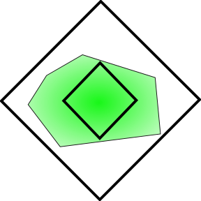
- Equivalently, make the `d`-polytope `P(A) := \{ x : {:|\|Ax\|\|:} _1 \le 1 \}` round or fat
Conditioning `A`, Motivation
- The conditioning here is an analog of orthogonalization, but for the `l_1` norm
- After orthogonalizing, have `|\|Ax\|\| _2 = |\|x|\| _2` for all `x`
- Conditioning relation is similar, but weaker
- Makes a "well-shaped" objective function for subgradient method
- Helpful also in sampling algorithm
- If `||x|| _1` is small, variance of sampled version of `||Ax-b|| _1`
must be also
- This step, plus `l_2` fit step, reduce effect of outliers
Conditioning `A`, in more detail
- Make columns of `A` orthogonal, scale so that `l_1` norm is one
- "Condition" is now `sqrt n`, will reduce to `d sqrt d`
- Apply ellipsoid method to "condition" `A` further
- Find Loewner-John ellipsoid pair
- Or, transform `P(A)` so that it is nested between concentric balls
- Faster because of first step
- Fast enough in `n gg d` regime
Overview of Algorithms, again
- Condition `A`, that is, make `{:|\|Ax\|\|:} _1 approx {:|\|x|\|:} _1` for all `x`
- Find `l_2` fit, subtract from `b` (change of variable)
- Apply modified subgradient algorithm, find `x_c` so that
`{:|\|Ax_c - b\|\|:} _1` no more than twice opt
- Either
- Apply subgradient algorithm more
- Or take weighted random sample of points, solve
Subgradients
- The function `F(x) equiv |\|Ax - b\|\| _1` is piecewise-linear,
so it has a gradient "almost everywhere"
- That gradient is `A^T sgn(Ax-b)`
- That is, a signed combination of the rows of `A`
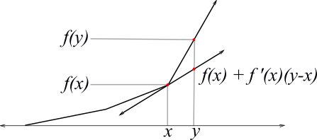
- At breakpoints of `F(x)`, gradient is undefined, but for any `x` and `y`,
`F(y) \ge F(x) + (y-x)^T A^T sgn(Ax-b)`
- That is, `A^T sgn(Ax-b)` is a subgradient, a member of the set `\del F(x)`
- Gradient for least squares is `A^T(Ax-b)`; setting this to zero gives "normal equations"
Subgradient Descent Method
- In particular, if `hat x equiv argmin _x F(x)`, then
`0 \le F(x) - F(hat x) \le (x - hat x)^T A^T sgn(Ax-b) = (hat x - x)^T(-A^T sgn(Ax-b))`
- So `G(x) equiv -A^T sgn(Ax-b)` points from `x` to `hat x`
- This subgradient property has been used for optimization
- Take `x_0 := 0`, and `x_{i+1} := x_i + sigma G(x_i)
- Here `sigma` is a multiplier to avoid overstepping
- Improvement in `F(x)` not guaranteed, that is, not a descent method
Subgradient Method: Stepsize
- Often `sigma` is taken as fixed, or slowly decreasing in some simple way
- Here, a careful program of `sigma` values allows provable convergence
- Can't just check for improvement: closer in `l_2`, but maybe not in function value
- Best stepsize depends on unknown ratio `{:F(x):}//{:F(hat x):}`
Subgradients Animation
sum= 0 rms= 0
How good is the subgradient?
- Let `theta` be the angle between `hat x - x` and `G(x)`
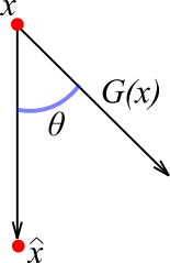
- How big is `cos theta`?
- We have
`{:|\|hat x - x|\|:} _2 {:|\| G(x)|\|:} _ 2 cos theta > F(x) - F(hat x)`
- How small are `|\| hat x - x |\| _2` and `|\| G(x)|\| _ 2`?
Subgradient Method: Using conditioning
- `{:|\| G(x)|\|:} _ 2 = {:|\| A^T sgn (Ax-b)|\|:} _ 2 le sqrt d`
- `{:|\|x|\|:} _ 1 > {:|\|Ax|\|:} _ 1` implies column sums of `A` are `le 1`.
- `{:|\|hat x - x|\|:} _2 \le d sqrt{d} (F(x) + F(hat x))`
- `{:|\|x-hat x|\|:} _2 \le {:|\|x-hat x|\|:} _1 \le d sqrt{d) {:|\|Ax-A hat x|\|:} _1 \le d sqrt{d)(F(x) + F(hat x))`
- So if `alpha equiv {:F(x):}//{:F(hat x):}`, then
`cos theta > (F(x) - F(hat x))/((sqrt(d))d sqrt{d)(F(x) + F(hat x))) > {:1/(d^2):}(alpha-1)/(alpha+1)`
Using the Subgradient
- `cos theta > (alpha-1)// {:d^2 (alpha+1):}`
- When `F(x) \gg F(hat x)`, `cos theta approx 1`, or `theta approx 0`, good
- When `F(x) approx F(hat x)`, not so good
- Leading to running time dependence `1//{:epsilon^2:}`
- Step length `{:|\|x-hat x|\|:} _2 cos theta \ge F(x)(1-{:1//alpha:})//sqrt(d)`
- Depends on `F(x)`, and on `alpha`, or an estimate of it
- Enough to use estimate smaller than `alpha`
- If estimate is below `alpha`, provable improvement in `F(x)`
- If above `alpha`, know that `alpha` can be reduced
Sampling Algorithm: Preprocessing
- Condition `A` using the ellipsoid method
- For applying subgradient algorithm, and useful for sampling
- Use subgradient algorithm to find `x'` with `{:|\|Ax'-b|\|:} _1 \le 2 {:|\|A hat x - b|\|:} _1`
- Replace `b` by `b-Ax'` (change of variable)
- Result is no "outliers"
Sampling and Solving
- Construct a diagonal `n times n` matrix `Z` to sample about rows of `A` and `b_i`
- Matrix `Z` will choose about `r` rows
- With choose `i`, and make `Z_{ii} gt 0`, with probability prop. to length of `a_{i cdot}`
- `f_i equiv {:|b_i|:} + {:|\|a_{i cdot}|\|:} _1`
- `W equiv sum_i f_i`
- `p_i equiv min \{ 1, r f_i//W \}
- Choose `y_i = 1` with probability `p_i`, `0` otherwise
- `Z_{ii} = y_i/p_i`
- Having sampled, solve: minimize `{:|\| Z(Ax-b)|\|:} _1`
Sampling Algorithm: Why it works
- `EZ = I`, and `E {:|\| Z(Ax-b)|\|:} _1 = {:|\| Ax-b|\|:} _1` for any given `x`
- Expected number of nonzero `Z_{ii}` is `r`
- Apply tail estimates, `X_i = Z_{ii}{:|b_i - a_{i cdot} x|:}`
- `sum_i E[(Z_{ii}{:|b_i - a_{i cdot} x|:})^2] approx {:|\| Ax -b |\|:} _1 ^2`
- That is, sum of squares within a constant factor of square of expectation
- Conditioning of `A` implies `f_i = {:|b_i|:} + {:|\|a_{i cdot}|\|:} _1`
is a good estimator of `|b_i - a_{i cdot} x| |\|x|\| _\infty`, on average
- Result is that, with high probability, `{:|\| Z(Ax-b)|\|:} _1 approx {:|\| Ax-b|\|:} _1`
Bernstein Bounds
- Use tail estimates of Maurer03, MO3:
- Given `X_i ge 0`, `i=1...n`, independent random variables
- Let `S = sum_i X_i`, then for any `t ge 0`,
`log Prob\{S le ES -t\} \le {:{:-t^2:}//{:2 sum_i EX_i^2:}:}`
- Tail estimate of Bernstein46:
- if also for some `M`, `X_i le EX_i + M`, then
`log Prob\{S ge ES + t\} \le {:{:-t^2:}//2(tM//3 + sum_i EX_i^2):}`
Coresets (motivation)
- One motivation here: are there coresets for `l_1` regression?
- Coreset for smallest ball problem:
- Given set of points `S` and `epsilon>0`
- there is `C subset S` of size ` lceiling 1//epsilon rceiling`, such that
- the smallest ball containing `C`, expanded by `1+epsilon`, contains `S`
- Independent of `|S|`, and even the dimension (!)
Coresets: uses
- Useful for `k`-center problem and others
- Similar results for approximating many geometric problems (but coresets may be larger)
- Here: sample taken by sampling algorithm is a kind of coreset
- Size `d^{O(1)}/epsilon^2`
Conclusion
- Provable results, plausible algorithms
- Can the ellipsoid method be avoided?
- Repeatedly apply subgradient algorithm to columns of `A`
- Remove linear combinations to make `l_1` residual small
- Apply to other regression schemes?
- Remove `log n` term?